Clipping and geometric operations for spherical polygons.
If you use npm, npm install d3-geo-polygon. You can also download the latest release on GitHub. For vanilla HTML in modern browsers, import d3-geo-polygon from Skypack:
<script type="module">
import {geoCubic} from "https://cdn.skypack.dev/d3-geo-polygon@2";
const projection = geoCubic();
</script>
For legacy environments, you can load d3-geo-projection’s UMD bundle from an npm-based CDN such as jsDelivr; a d3 global is exported:
<script src="https://cdn.jsdelivr.net/npm/d3-array@3"></script>
<script src="https://cdn.jsdelivr.net/npm/d3-geo@3"></script>
<script src="https://cdn.jsdelivr.net/npm/d3-geo-polygon@2"></script>
<script>

const projection = d3.geoCubic();

</script>
This module introduces a handful of additional projections. It can also be used to clip a projection with an arbitrary polygon:
const projection = d3.geoEquirectangular()
  .preclip(d3.geoClipPolygon({
    type: "Polygon",
    coordinates: [[[-10, -10], [-10, 10], [10, 10], [10, -10], [-10, -10]]]
}));# d3.geoClipPolygon(polygon) · Source, Examples
Given a GeoJSON polygon or multipolygon, returns a clip function suitable for projection.preclip.
# clip.polygon([geometry])
If geometry is specified, sets the clipping polygon to the geometry and returns a new clip function. Otherwise returns the clipping polygon.
# clip.clipPoint([clipPoint])
Whether the projection should clip points. If clipPoint is false, the clip function only clips line and polygon geometries. If clipPoint is true, points outside the clipping polygon are not projected. Typically set to false when the projection covers the whole sphere, to make sure that all points —even those on the edge of the clipping polygon— get projected.
# d3.geoIntersectArc(arcs) · Source, Examples
Given two spherical arcs [point0, point1] and [point2, point3], returns their intersection, or undefined if there is none. See “Spherical Intersection”.
d3-geo-polygon adds polygon clipping to the polyhedral and interrupted projections from d3-geo-projection. Thus, it supersedes the following symbols:
# d3.geoPolyhedral(tree, face) · Source, Examples
Defines a new polyhedral projection. The tree is a spanning tree of polygon face nodes; each node is assigned a node.transform matrix. The face function returns the appropriate node for a given lambda and phi in radians.
Polyhedral projections’ default clipPoint depends on whether the clipping polygon covers the whole sphere. When the polygon’s area is almost complete (larger than 4π minus .1 steradian), clipPoint is set to false, and all point geometries are displayed, even if they (technically) fall outside the clipping polygon. For smaller polygons, clipPoint defaults to true, thus hiding points outside the clipping region.
# polyhedral.tree() returns the spanning tree of the polyhedron, from which one can infer the faces’ centers, polygons, shared edges etc.
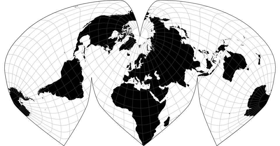
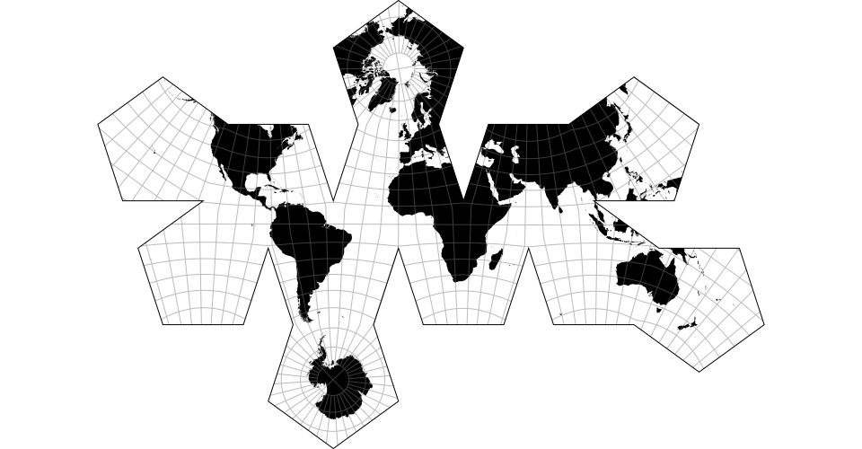
# d3.geoPolyhedralButterfly() · Source
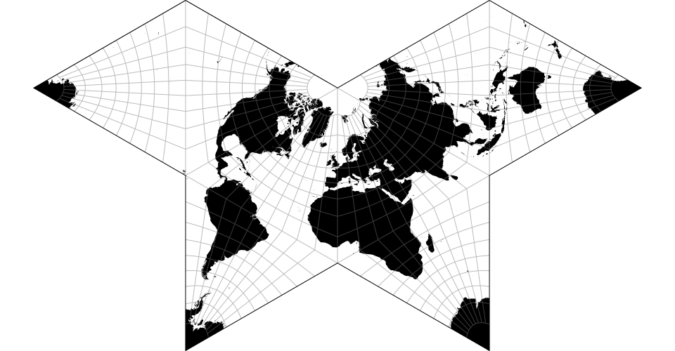
The gnomonic butterfly projection.
# d3.geoPolyhedralCollignon() · Source
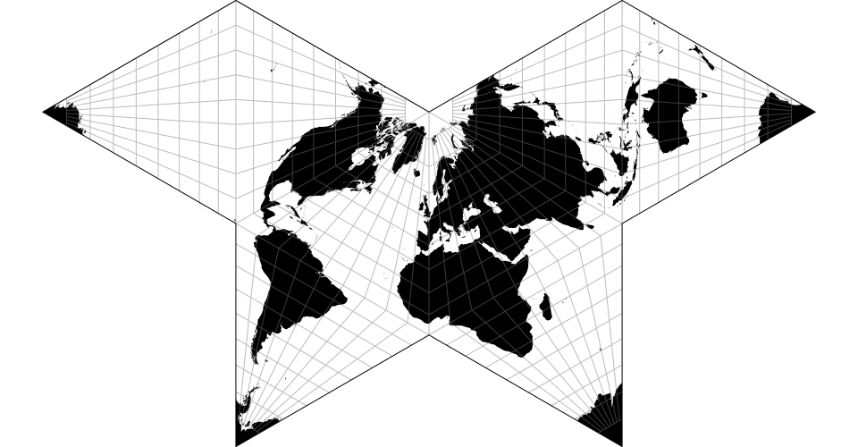
The Collignon butterfly projection.
# d3.geoPolyhedralWaterman() · Source
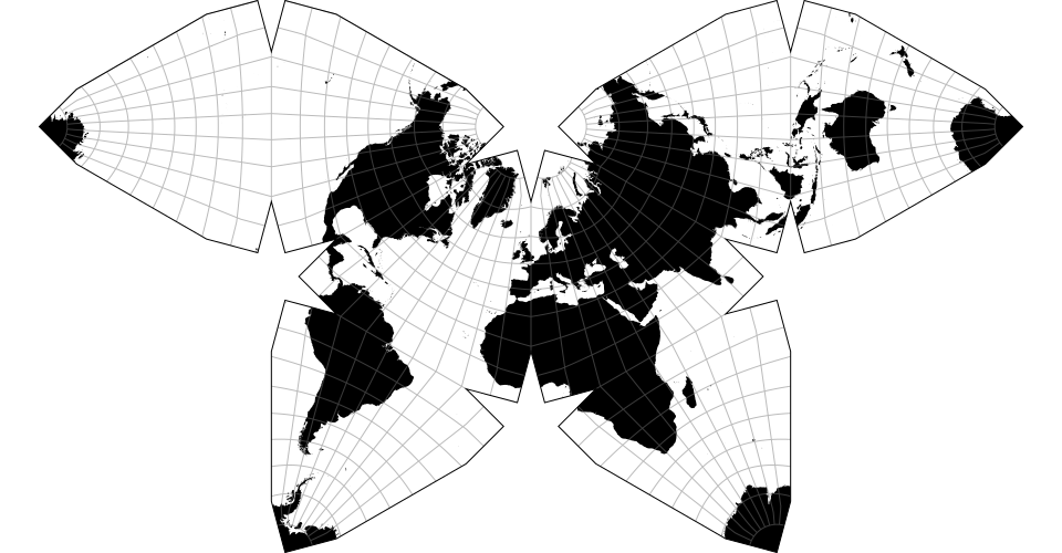
A butterfly projection inspired by Steve Waterman’s design.
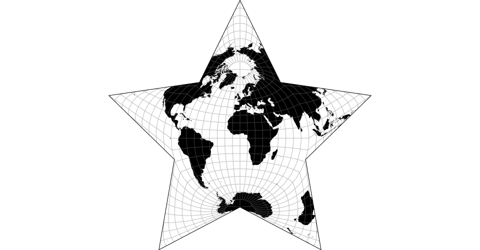
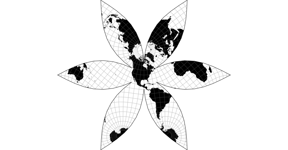
The Berghaus projection.
The Gingery projection.
The HEALPix projection.
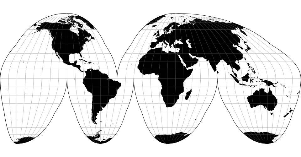
# d3.geoInterruptedBoggs · Source
Bogg’s interrupted eumorphic projection.
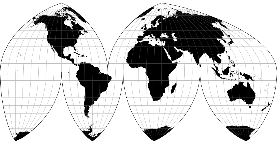
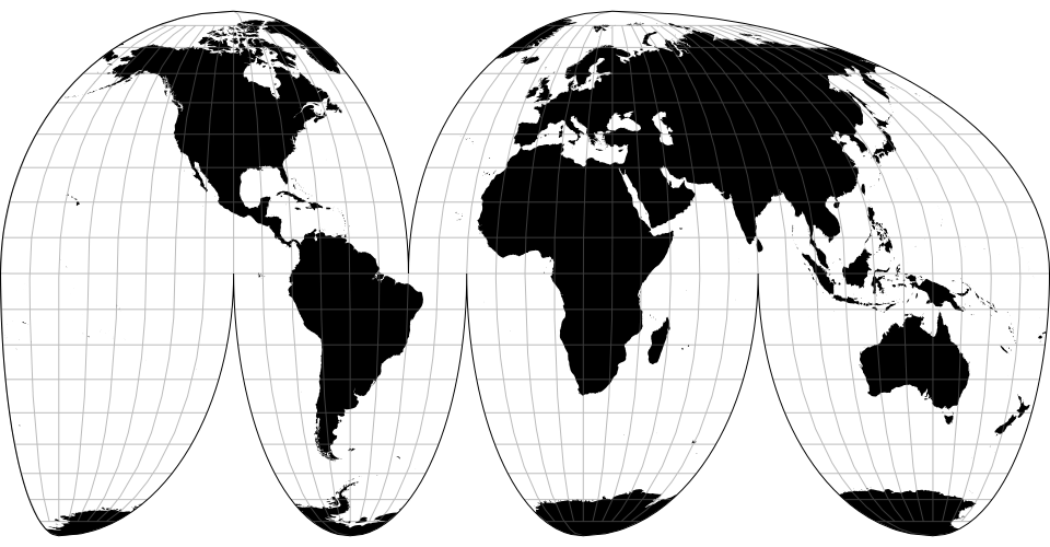
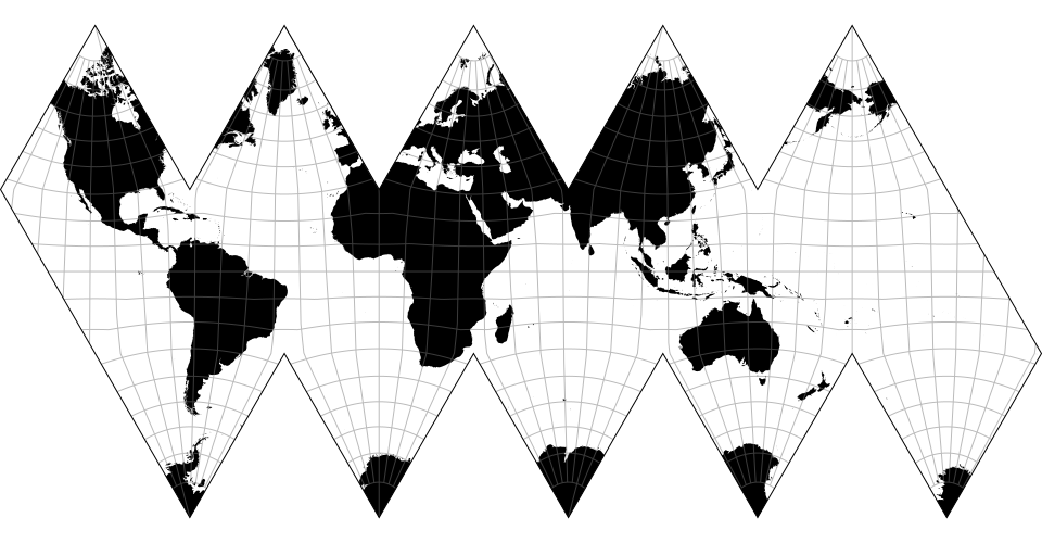
# d3.geoInterruptedHomolosine · Source
Goode’s interrupted homolosine projection.
# d3.geoInterruptedMollweide · Source
Goode’s interrupted Mollweide projection.
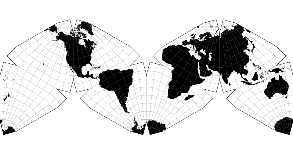
# d3.geoInterruptedMollweideHemispheres · Source
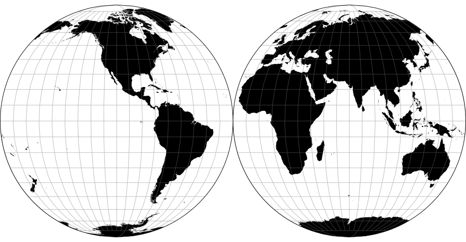
The Mollweide projection interrupted into two (equal-area) hemispheres.
# d3.geoInterruptedSinuMollweide · Source
Alan K. Philbrick’s interrupted sinu-Mollweide projection.
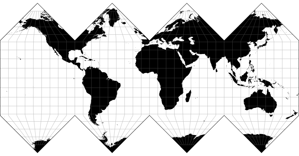
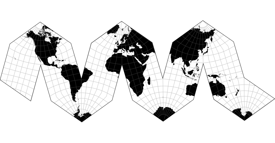
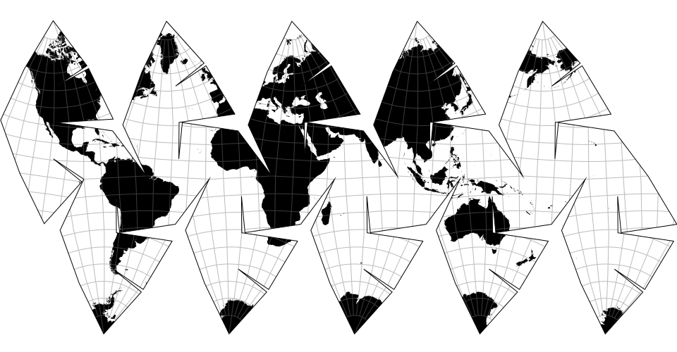
# d3.geoInterruptedSinusoidal · Source
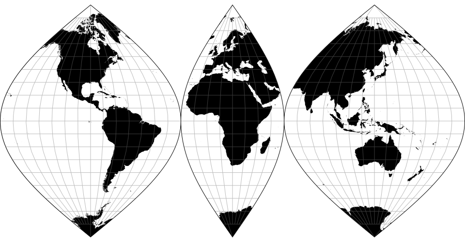
An interrupted sinusoidal projection with asymmetrical lobe boundaries.
# d3.geoTwoPointEquidistant(point0, point1) · Source
The two-point equidistant projection, displaying 99.9996% of the sphere thanks to polygon clipping.
# d3.geoTwoPointEquidistantUsa() · Source
The two-point equidistant projection with points [-158°, 21.5°] and [-77°, 39°], approximately representing Honolulu, HI and Washington, D.C.
New projections are introduced:
# d3.geoPolyhedralVoronoi([parents], [polygons], [faceProjection], [faceFind]) · Source
Returns a polyhedral projection based on the polygons, arranged in a tree.
The tree is specified by passing parents, an array of indices indicating the parent of each face. The root of the tree is the first face without a parent (with the array typically specifying -1).
polygons are a GeoJSON FeatureCollection of geoVoronoi cells, which should indicate the corresponding sites (see d3-geo-voronoi). An optional faceProjection is passed to d3.geoPolyhedral() -- note that the gnomonic projection on the polygons’ sites is the only faceProjection that works in the general case.
The .parents([parents]), .polygons([polygons]), .faceProjection([faceProjection]) set and read the corresponding options. Use .faceFind(voronoi.find) for faster results.
# d3.geoCubic() · Source, Examples
The cubic projection.
# d3.geoDodecahedral() · Source, Examples
The pentagonal dodecahedral projection.
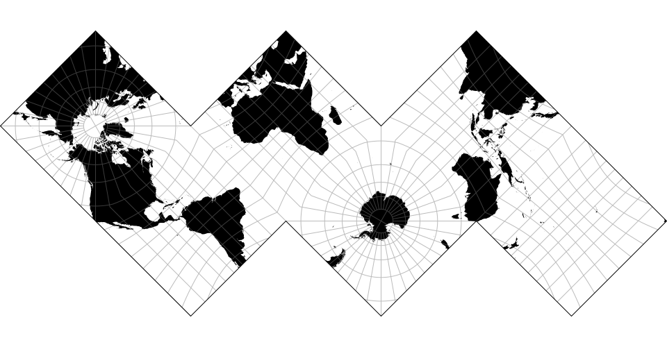
# d3.geoRhombic() · Source, Examples
The rhombic dodecahedral projection.
# d3.geoDeltoidal() · Source, Examples
The deltoidal hexecontahedral projection.
# d3.geoIcosahedral() · Source, Examples
The icosahedral projection.
# d3.geoAirocean() · Source, Examples
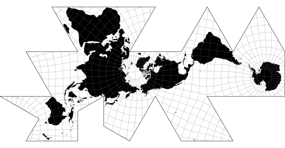
Buckminster Fuller’s Airocean projection (also known as “Dymaxion”), based on a very specific arrangement of the icosahedron which allows continuous continent shapes. Fuller’s triangle transformation, as formulated by Robert W. Gray (and implemented by Philippe Rivière), makes the projection almost equal-area.
# d3.geoCahillKeyes() · Source, Examples
# d3.geoCahillKeyes
The Cahill-Keyes projection, designed by Gene Keyes (1975), is built on Bernard J. S. Cahill’s 1909 octant design. Implementation by Mary Jo Graça (2011), ported to D3 by Enrico Spinielli (2013).
# d3.geoImago() · Source, Examples
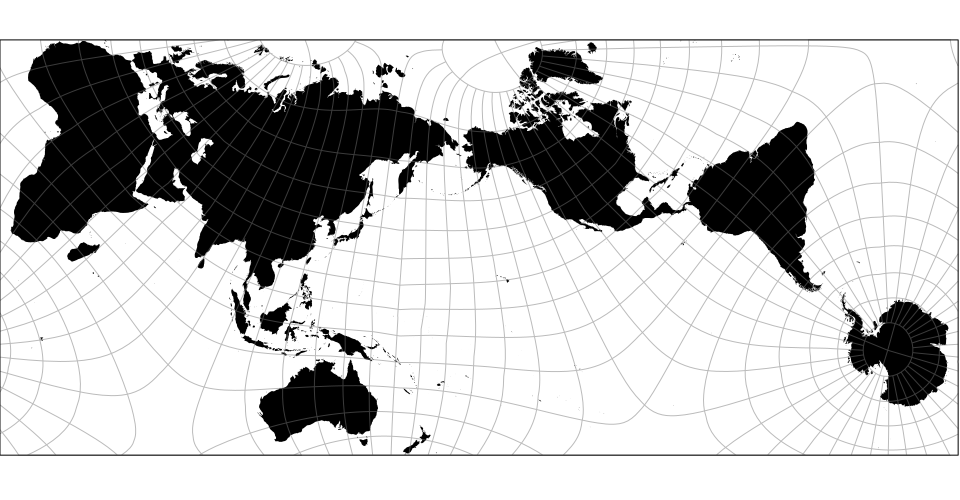
The Imago projection, engineered by Justin Kunimune (2017), is inspired by Hajime Narukawa’s AuthaGraph design (1999).
# imago.k([k])
Exponent. Useful values include 0.59 (default, minimizes angular distortion of the continents), 0.68 (gives the closest approximation of the AuthaGraph) and 0.72 (prevents kinks in the graticule).
# imago.shift([shift])
Horizontal shift. Defaults to 1.16.
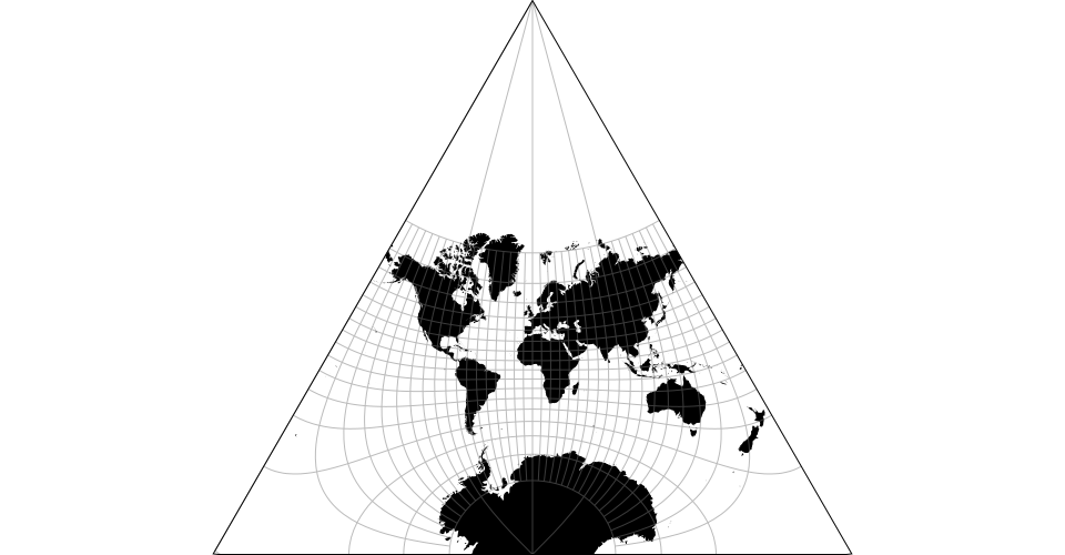
# d3.geoTetrahedralLee() · Source, Examples
# d3.geoLeeRaw
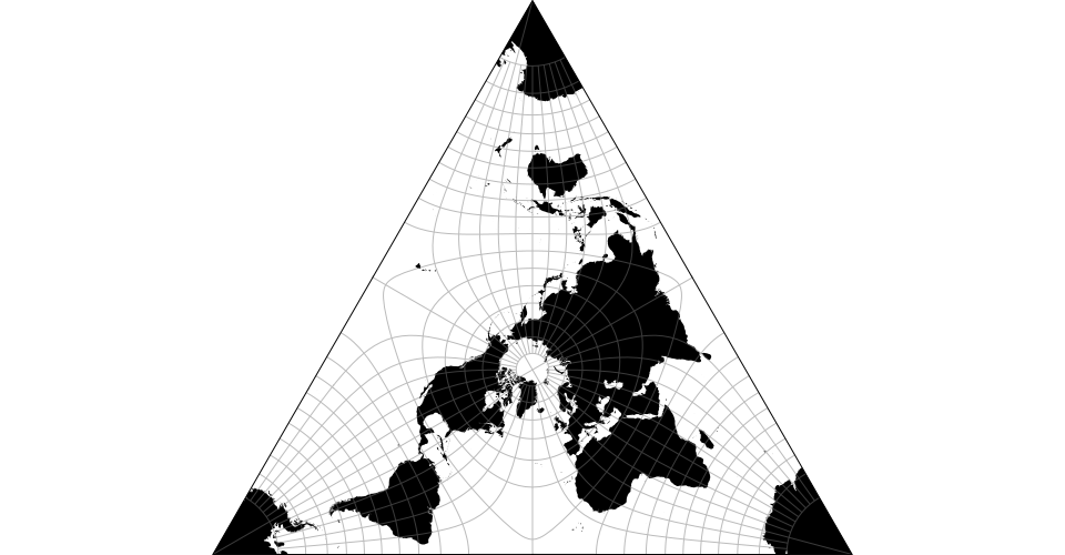
Lee’s tetrahedral conformal projection.
# Default angle is +30°, apex up (-30° for base up, apex down).
Default aspect uses projection.rotate([30, 180]) and has the North Pole at the triangle’s center -- use projection.rotate([-30, 0]) for the South aspect.
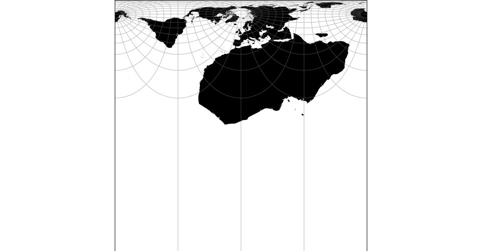
# d3.geoCox() · Source, Examples
# d3.geoCoxRaw
The Cox conformal projection.
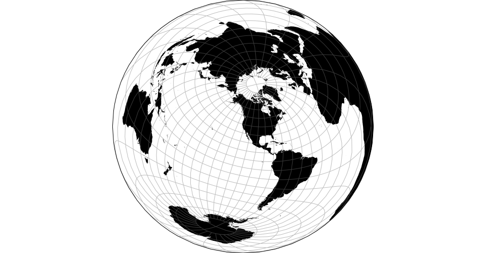
# d3.geoComplexLog([planarProjectionRaw[, cutoffLatitude]]) · Source, Example
# d3.geoComplexLogRaw([planarProjectionRaw])
Complex logarithmic view. This projection is based on the papers by Joachim Böttger et al.:
- Detail‐In‐Context Visualization for Satellite Imagery (2008)
- Complex Logarithmic Views for Small Details in Large Contexts (2006)
The specified raw projection planarProjectionRaw is used to project onto the complex plane on which the complex logarithm is applied. Recommended are azimuthal equal-area (default) or azimuthal equidistant.
cutoffLatitude is the latitude relative to the projection center at which to cutoff/clip the projection, lower values result in more detail around the projection center. Value must be < 0 because complex log projects the origin to infinity.
# complexLog.planarProjectionRaw([projectionRaw])
If projectionRaw is specified, sets the planar raw projection. See above. If projectionRaw is not specified, returns the current planar raw projection.
# complexLog.cutoffLatitude([latitude])
If latitude is specified, sets the cutoff latitude. See above. If latitude is not specified, returns the current cutoff latitude.