The process of self driving can be divided into 3 big parts: Data Input, Processing, Motion Planning. The perpose of this github repository is to implement this process. It will be composed of 4 different parts: (1) Vehicle Modeling (2) Kalman Filter Implementation (3) Camera Image Processing (4) Motion Planning.
To analyze the vehicle's movement, we need to model the vehicle and figure out what kind of factors effect the vehicle in which kind of result. The vehicle modeling can by divided in 2 different aspects: Kinematic Modeling and Dynamic Modeling.
Kinematic Modeling is used especially at low speeds when the accelerations are not significant to capture the motion of a vehicle. In most cases, it is sufficient to look only at kinamic models of vehicles. One of the most famous model is the bicycle model, which is implemented in the code. Using the bicycle model, we can make the bicycle to move in the direction as we want by controling the steering angle speed (the vehicle speed is fixed, hence it is used when accelerations are not signifcant). The result can show like this:

When we need to include knowledge of the forces and moments acting on the vehicle, we're performing Dynamic Modeling. In this model, we have to control the throttle and break of the vehicle to make the vehicle to move in the required speed on the road. You can check the implemention of the vehicle speed on the code.
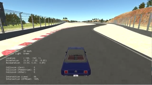
Using the above 2 models, we can control the vehicle to run on the required trajectory, as you can imagine the car have a steering wheel, an accelerator (throttle), and break. The final implementation of the vehicle modeling is about making a 3d simualator using the CARLA Unreal game engine.
The required path is provided as the data, and we can use this in the implement of pure pursuit or stanley method. Check the result of the development in the following video :
To make the vehicle to move as we expect, we have to understand exactly about the parameters that effect the movement of the vehicles. The modeling method can help this, and must be applied in the autonous driving system.
In the self-driving car system, there must be data to recognize where the vehicle itself is located in the real world, or detect obstacles that the vehicle must avoid, etc. For these operations, the car needs to have sensors (just like the human beings), and collect information of the environment. There are many types of data that can be used in the self driving car system, and in this project we will figure out about how to address with the 2 mostly used data tyoe in the industry: the LIDAR sensor data, and images collected by the Camera. In Section 2. Kalman Filter, we will discribe how to use the LIDAR sensor data, and in 3. Visual Perceptions, we will talk about image processing.
Not only in self-driving, but also in many other various fields use different types of sensors for data production. But unfortunally, the data value can not be used directly because of the uncertaincy of the sensor itself. For example, many people know the formula below, the Ohm's Rule:
V = IR
But actually when we measure the voltage and current between the resister several times, we will recognize that values does not show that R is always the same, which means that there is a noise value between the 'real resist' and 'expected resist'. So the fomular above can be deformed as below:
R = V / I + a
where a is the noise value which is usually supposed to have a standard normal distribution. In VoltageProblem.py, we implement the least square error method to control this error, and predict the exact value that we want.
The self driving car needs to know where itself is in the world space, and we can think 2 different solutions to tackle this problem.
The first method is using the vehicle modeling technique, similar to what we have done in section 1. Using the value of the accelation and steering wheel angle, we can predict where the vehicle positions in the world time by time. But the problem of this method is that it is only the predicted location, which means it can be correct only when the acceleration and steering wheel can effect the vehicle, but in real world there can be hundreds of other types of forces, such as the land slope, wind, or even an earthquake, etc, and these make the predicted location to be wrong. To cover this by modeling, we need to model not only the vehicle itself, but also the entire world which have enormous variety of forces, that seems to be clearly impossible.
The second one is using sensor data, such as GPS, Lidar, etc. It seems to be more easy than modeling the entire world (the first method), but as mentioned at section, sensors do not show the 'exact' value because of the noise, and this phenomenon equally happens to location problem. Another problem of using sensor data in localiztion problem is that the data is in serial, which means that it is a different problem mentioned in the voltage problem which gives all the measured data at once. In localizing, the data accumulates in every period, making the least square error useless (before deforming).
Kalman filter can be called as the hybrid method of these 2. Kalman filter first predicts the location using the vehicle motion model as the first method, and then corrects the predicted location by the measurement model addressed in the second method. The code implemented in this section notes about the estimation of the vehicle trajectory using the EKF (Extended Kalman Filter) which is an extended version of Kalman filter used when the data is non linear. The ground truth data shows the trajectory as below :

The mission of this code is to estimate the trajectory as closed as possible to the ground truth data, using the starting point, LIDAR sensor data, linear and angular velocity odometry data. We need to use linear and angular velocity odometry value in the motion model, and the LIDAR sensor data in the measurment model. The results are showm below :

Using only 1 LIDAR camera can be dangerous due to the sensor malfunction, noise, etc. The solution of this problem is quite simple : use more than 1 LIDAR camera. We can also think that we can collect different types of sensors for more accurate results by processing various types of data. This operation is called sensor calibration.
In this section, we will simulate the calibration of 3 different types of sensors LIDAR, GNSS and IMU using the Error State Extended Kalman Filter (ES-EKF). The mission is the same as the above ekf implement and there will be different three tests. The results are shown below :

The first figure shows the estimated trajectory figured out by es-ekf when all the sensors are operating normally. The second figures shows when the LIDAR camera is supposed to be slightly declined compared to the ordinary state and rectified by changing the covariance of the LIDAR sensor and IMU sensor noise. The third figure is the result of the test when all external positioning information (from GPS and LIDAR) is lost for a short period of time.
In this section we learned about how the vehicle can estimate itself state (position). Now the estimated position is ready, and this will be used in the motion planning stage.
Camera is a fruitful source of data that can be used in various ways. In this section, we will talk about (1) how to detect a target object on road using stereo camera, (2) localization using continuous scenes from camera (3) environment perception.
Using 2 cameras arranged on the same epipoly line (just like the human eyes), we can calculate how far the appeared objects on the lens are from the cameras which is called depth. In addition, using the cross correlation method, we can detect obstacles on the road and prevent collisions by prevision of the depth value.
In the depository, there will be given two images, one is the left side camera's picture, and the other is the right side's. Using these images, we will first construct the disparity map and then develop it into the depth map.


Finally, we can detect the distance from the vehicle to the objects using cross correlation and the depth map. In this example, we will to detect the motorcycle and how much far it is from the driver. The results are shown below.

The twinkling point in the picture is the discription where the detected object locates in the image.
Using the depth maps of each frame, we can track the maneuver of the vehicle. To do this we will first detect the feature points of frame i and frame i+1 and match the features by pairing the same feature points.

Using the matches and the depth maps of frame i an i+1 , we can estimate how mush far the vehicle moved, how much fast the vehicle have rotated.

When we apply this into all available frames, we can approximate to the real trajectory of the vehicle.

The depth map is not only useful in trajectory estimation, but also in environment perception. This means the detection of the road, objects, traffic lights, signatures, etc. In this sub section we will check how to calculate the plane equation in world coordinates and where obstacles are placed. A frame will be offered with the segementation data and the depth map which are supposed to be processed before detection. To calculate the road's plane equation, we first need to convert all the pixel's uv coordinated into world coordinates. This can be done by using the image size and the depth value of the pixel we want to convert. After this conversion, we have to distinguish which world coordinates belongs to the road plane equation using the segmentation data. We can choose random 3 points of the whole set of these distinguished road points, and use it to calculate the equation. Of course, only 1 try of random selection is not enough to claim that the equation is fully correct, so we do this several time and decrease the error. Now we can estimate where the self-driving car can physically travel. During the execution of the implement, you can get a plot like this:

The left is the given frame, and the right is the 3d plot of where the vehicle can move. The boxes are the match of these two images.
After the process of the road plane detection, we now need to need to know where the vehicle actually can move, not physically but legally, by detecting the lanes. We will learn what apis are useful to detect the lanes, add finally construct the extrapolated lines.
The final task of this section is to detect the obstacles on the road, similar what we have done in the first subsection. The different point is that now we cannot use the template image, instead the object detection results (progressed by CNNN) and the segementation data. We will distinguish important objects from the detection and locate where the objects are, again, using depth map and segmentation. The results will show like this:

Finishing the perception stage, now the self-driving car is able to plan where to go. This planning stage can be divided into mission planning, behavior planning, and local planning. This section introduces what are the differences between these planners, and how to develop them.
In previous sections, to know where the vehicle is, we have used a visual method, but there is a more easier approach using the LIDAR sensor. Using the LIDAR sensor we can confortably construct an occupancy grid to know where obstacles are on the road. An occupancy grid is a grid that each point shows whether it is occupied by some object. This subsection show the implement of the occpancy grid construction using inverse measurement model. The results will show as below:


Mission planning means the deciding the navigation from point A to B on the map. It is the most high level of the planning system, and the goal is to find the most less costed path between the 2 points. Dijkstra algoritm is one famous method to figure out the most least costed path. This subsection introduces the implementation of this method. We will understand how to use the osmnx package and compare the implemented results with the ground truth data of osmnx. The dijkstra result will show like this:

In this subsection, we will implement the whole process of motion planning, except the mission planner that is already introduced above. There are many stages, including the behavior planner, local planner, path planner, etc. We need to understand every part of the planner to make a non-collision, safe, and fast self driving vehicle. The result is shown as a video clip below:
